How to create drop-down list in Excel

Have you ever created drop-down lists in Excel? It helps your work more efficient.

Here's some merits to use it.

• Prevent mistyping
• Don't have to remember what you enter
• Enter contents with the same format

Especially, it's useful when you sort data with filter.

You can learn how to create drop-down lists, using data validation and refering to data in other worksheets.

What is a drop-down list?

A drop-down list is defined like this.

It is a way to select an item on operating screen of OS with GUI or Web pages, only one item can be selected from several items.
When the button is clicked, the list of items are displayed. It's also called pull-down list.

In Excel, it's the list that is shown by clicking ▼ and you can choose one item from there. It's also called drop-down menu or pull-down list.

How to create a drop-down list

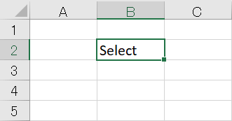
Enter "Select" in a cell which you want to create a pull-down list.

STEP1 Select the Data Validation

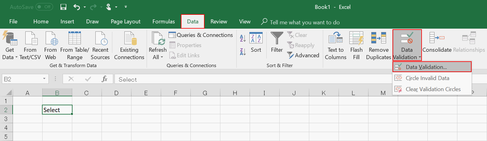
Select【Data Validation】under the【Data】 tab.

STEP2 Select the List in the dialog box

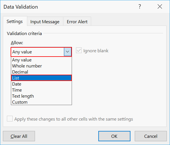
Click【Any value】and select 【List】 in the Data Validation dialog box.

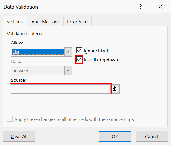
Make sure that 【In cell dropdown】is checked and【Source】is empty.

STEP3 Enter values in 【Source】

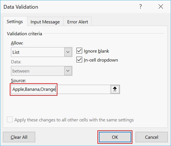
Enter values which you want to show in the list in【Source】entry box. In this example, we enter "Apple", "Banana", "Orange". These words must be separated by commas. Then click 【OK】.

Complete

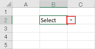
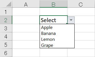
【▼】apper on the right of the cell, when "Select" cell is selected.

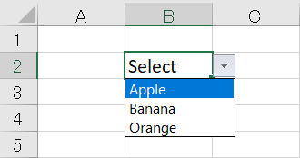
When【▼】is clicked, the drop-down list is shown. Then you can select a value from the list.

How to create a drop-down list refer to data in a worksheet

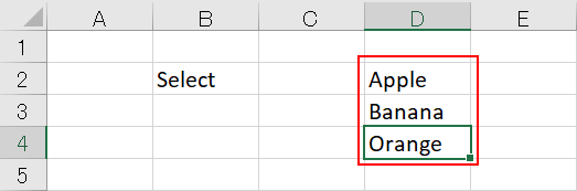
You can also create a drop-down list refer to the data in a worksheet. For the first, enter the list in the worksheet as seen above.

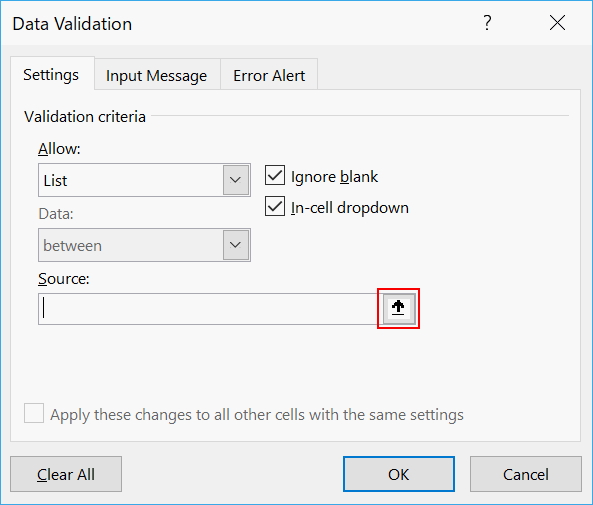
Open【Data Validation】dialog box as explained above, and click the icon which placed the right of the source entry box.

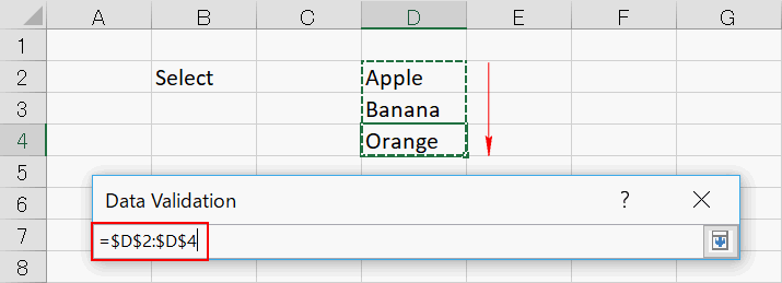
Drag-select the data.How to edit a drop-down list.

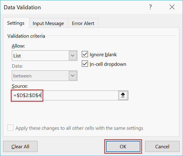
Then the selected area is entered in【Source】. In this case, "$D2$2:$D$4" is entered. Click 【OK】.

How to edit a drop-down list

Revise a list

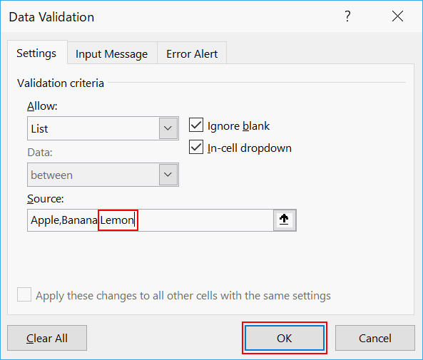
Select the cell which is applied the drop-down list which you want to revise and open 【Data Validation】dialog box. Then you can change the values in【Source】.

In this case, we change it from "Orange" to "Lemon".

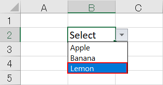
The revision is reflected on the list.

Add values in a list

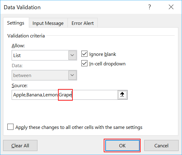
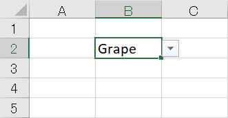
Add "Grape" in【Source】.

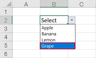
It's refrected to the list.

Clear a list

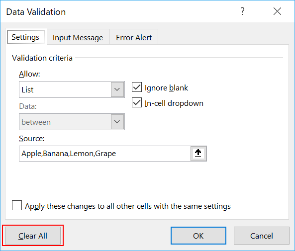
Open 【Data Validation】dialog box and click 【Clear All】.

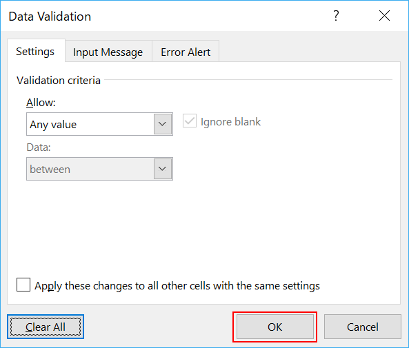
The setting is back to the default. Click【OK】, then the cell is back to normal.

Select a value by using a keyboard

It is hassle to click 【▼】every time when you select a value. The shortcut key makes it easier.

Press Alt + ↓ and the drop-doen list is shown.

Press ↑ or ↓ to select. Press Home to move the top, End to move to the last.

Press Enter to complete, then the value is entered in the active cell.

Advanced functions

Refer to data in another worksheet

You already learned to creat a drop-down list referring to data in the same worksheet. Now you can learn to create a drop-down list referring to data in another worksheet.

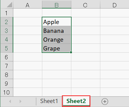
Drag-select data in another sheet

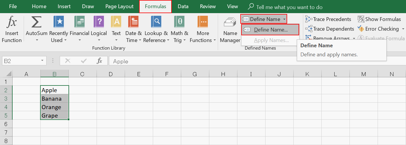
Click 【Define Name】under the【Formulas】tab.

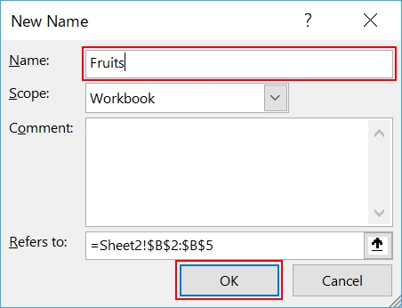
Enter name which you want to define. In this case, we enter "Fruits". Then click 【OK】.

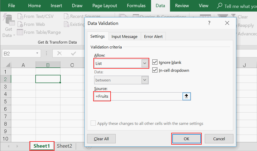
Go to the worksheet which you want to create a drop-down list and open【Data Validation】dialog box. Enter "=Fruits" in 【Source】and click 【OK】.

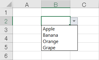
The data in Sheet2 appers as the drop-down list in Sheet1.

Counting cells which are selected from drop-down list

Here we introduce a way to count drop-downed cells.

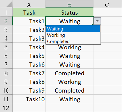
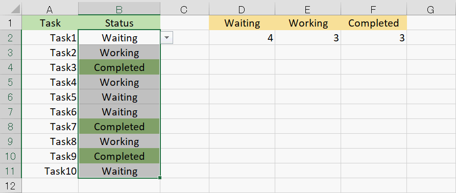
For example, applying the drop-down lists "Waiting / Working / Completed" for each task, when you manage tasks in Excel.

When you just select each status from drop-down list, it's hard to know how many tasks are in waiting. Let's diaplay the number in each status.

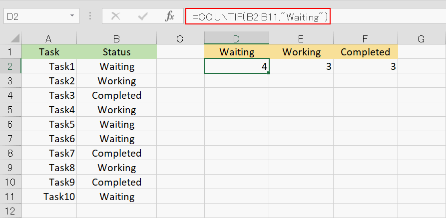
Enter "=COUNTIF(B2:B11,"Waiting")" in D2, "=COUNTIF(B2:B11,"Working")" in E2, "=COUNTIF(B2:B11,"Completed")" in F2.

Now the numbers of tasks are shown in each status.

We used COUNTIF function to count the number of each status. It works when you insert "=COUNTIF(range, criteria)".

Color with Conditional formatting function

When you want to classify the items, you can use 【Conditional Formatting】.

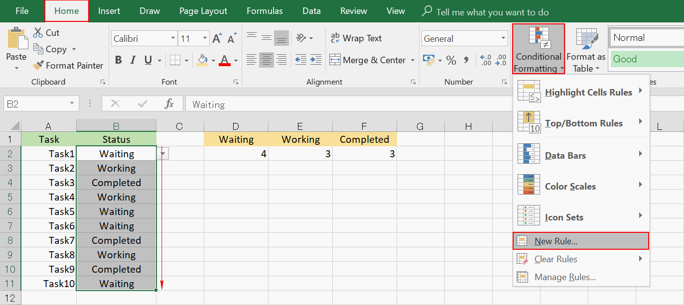
Drag-select the area which you want to classify. Then select【New Rule】under【Conditional Formatting】in【Home】tab.

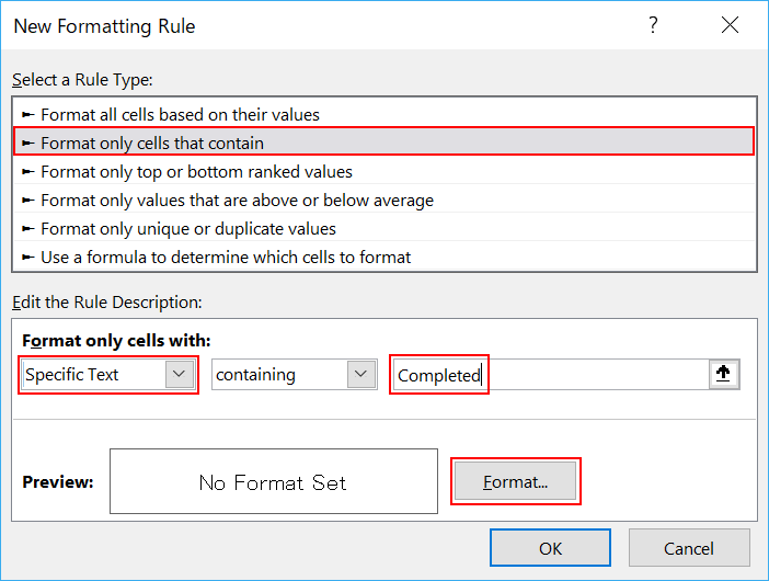
Select 【Format only cells that contain】and change 【Cell Value】to【Specific Text】.

Enter the words which you want to classify in the box next to 【containing】. In this case, enter "Completed".

Then click 【Format...】.

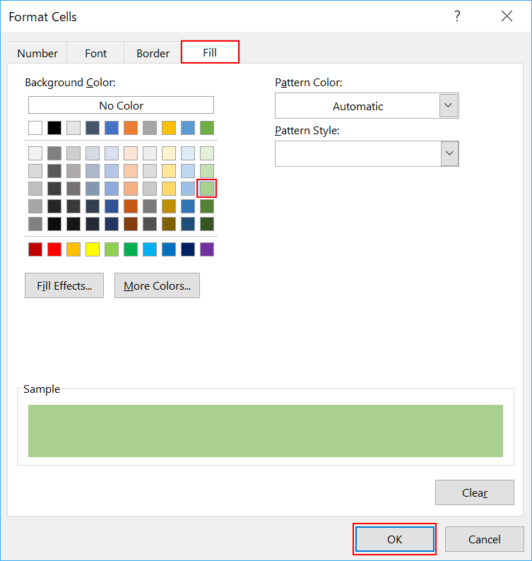
【Format Cells】dialog box is diaplayed.

Select 【Fill】tab and select the color. In this case, we chose yellow green. Then click【OK】.

When "Completed" are selected, cells which applied the conditional format will be filled the color.